সেগমেন্ট ট্রি#
সেগমেন্ট ট্রি হল একটি ডেটা স্ট্রাকচার যা অ্যারে ইন্টারভালের তথ্য একটি ট্রির আকারে সংরক্ষণ করে। এটি একটি অ্যারের উপর রেঞ্জ কোয়েরিতে দক্ষভাবে উত্তর দিতে দেয়, এবং একই সাথে অ্যারে দ্রুত পরিবর্তনের জন্য যথেষ্ট নমনীয়। এতে $a[l \dots r]$ ক্রমাগত অ্যারে উপাদানের যোগফল খুঁজে পাওয়া বা এই ধরনের একটি রেঞ্জে ন্যূনতম উপাদান $O(\log n)$ সময়ে খুঁজে পাওয়া অন্তর্ভুক্ত। এই ধরনের কোয়েরিতে উত্তর দেওয়ার মধ্যে, সেগমেন্ট ট্রি একটি উপাদান প্রতিস্থাপন করে অথবা সম্পূর্ণ সাবসেগমেন্টের উপাদান পরিবর্তন করে (যেমন সমস্ত উপাদান $a[l \dots r]$ যেকোনো মান নির্ধারণ করা, বা সাবসেগমেন্টের সমস্ত উপাদানে একটি মান যোগ করা) অ্যারে পরিবর্তন করতে দেয়।
সাধারণভাবে, সেগমেন্ট ট্রি একটি অত্যন্ত নমনীয় ডেটা স্ট্রাকচার, এবং এটির সাথে বিশাল সংখ্যক সমস্যা সমাধান করা যায়। অতিরিক্তভাবে, আরও জটিল অপারেশন প্রয়োগ এবং আরও জটিল কোয়েরির উত্তর দেওয়াও সম্ভব (দেখুন সেগমেন্ট ট্রির উন্নত সংস্করণ)। বিশেষত সেগমেন্ট ট্রি সহজেই বৃহত্তর মাত্রায় সাধারণীকৃত করা যায়। উদাহরণস্বরূপ, একটি দ্বি-মাত্রিক সেগমেন্ট ট্রির সাথে আপনি একটি প্রদত্ত ম্যাট্রিক্সের কিছু সাবরেক্ট্যাঙ্গেলের উপর সাম বা ন্যূনতম কোয়েরিতে $O(\log^2 n)$ সময়ে উত্তর দিতে পারেন।
সেগমেন্ট ট্রির একটি গুরুত্বপূর্ণ বৈশিষ্ট্য হল তাদের কেবল রৈখিক পরিমাণ মেমোরি প্রয়োজন। স্ট্যান্ডার্ড সেগমেন্ট ট্রি আকার $n$ এর একটি অ্যারেতে কাজ করার জন্য $4n$ ভার্টেক্স প্রয়োজন।
সেগমেন্ট ট্রির সহজতম রূপ#
সহজভাবে শুরু করতে, আমরা সেগমেন্ট ট্রির সহজতম রূপ বিবেচনা করি। আমরা সাম কোয়েরিতে দক্ষভাবে উত্তর দিতে চাই। আমাদের কাজের আনুষ্ঠানিক সংজ্ঞা হল: একটি অ্যারে $a[0 \dots n-1]$ দেওয়া হলে, সেগমেন্ট ট্রি অবশ্যই সূচক $l$ এবং $r$ এর মধ্যে উপাদানের যোগফল খুঁজে পেতে সক্ষম হতে হবে (অর্থাৎ যোগফল $\sum_{i=l}^r a[i]$ গণনা করা), এবং অ্যারেতে উপাদানের মান পরিবর্তন করতে সামলাতে হবে (অর্থাৎ $a[i] = x$ ফর্মের অ্যাসাইনমেন্ট সম্পাদন করা)। সেগমেন্ট ট্রি উভয় কোয়েরি $O(\log n)$ সময়ে প্রক্রিয়া করতে সক্ষম হতে হবে।
এটি সরল পদ্ধতির একটি উন্নতি। একটি সরল অ্যারে ইমপ্লিমেন্টেশন - শুধুমাত্র একটি সাধারণ অ্যারে ব্যবহার করা - উপাদান $O(1)$ এ আপডেট করতে পারে, কিন্তু প্রতিটি সাম কোয়েরি গণনা করতে $O(n)$ প্রয়োজন। এবং পূর্বনির্ধারিত প্রিফিক্স সাম সাম কোয়েরি $O(1)$ এ গণনা করতে পারে, কিন্তু একটি অ্যারে উপাদান আপডেট করতে প্রিফিক্স সামের $O(n)$ পরিবর্তন প্রয়োজন।
সেগমেন্ট ট্রির কাঠামো#
অ্যারে সেগমেন্টের ক্ষেত্রে আমরা একটি ডিভাইড অ্যান্ড কনকার পদ্ধতি অনুসরণ করতে পারি। আমরা সম্পূর্ণ অ্যারের উপাদানের যোগফল গণনা এবং সংরক্ষণ করি, অর্থাৎ সেগমেন্ট $a[0 \dots n-1]$ এর যোগফল। তারপর আমরা অ্যারেকে দুটি অংশে ভাগ করি $a[0 \dots (n-1)/2]$ এবং $a[(n+1)/2 \dots n-1]$ এবং প্রতিটি অর্ধ অংশের যোগফল গণনা এবং সংরক্ষণ করি। এই দুটি অর্ধ অংশের প্রত্যেকটি ক্রমে অর্ধেক করা হয়, এবং এভাবে চলে যতক্ষণ না সমস্ত সেগমেন্ট আকার $1$ এ পৌঁছায়।
আমরা এই সেগমেন্টগুলিকে একটি বাইনারি ট্রি তৈরি করার দৃষ্টিভঙ্গি থেকে দেখতে পারি: এই ট্রির রুট হল সেগমেন্ট $a[0 \dots n-1]$, এবং প্রতিটি ভার্টেক্স (লিফ ভার্টেক্স ছাড়া) ঠিক দুটি চাইল্ড ভার্টেক্স রয়েছে। এজন্যই ডেটা স্ট্রাকচারকে “সেগমেন্ট ট্রি” বলা হয়, যদিও বেশিরভাগ ইমপ্লিমেন্টেশনে ট্রিটি স্পষ্টভাবে নির্মিত হয় না (দেখুন ইমপ্লিমেন্টেশন)।
$a = [1, 3, -2, 8, -7]$ অ্যারের উপর এই ধরনের সেগমেন্ট ট্রির একটি ভিজ্যুয়াল উপস্থাপনা এখানে রয়েছে:
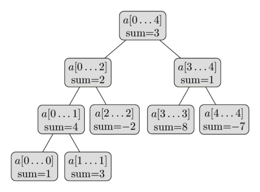
ডেটা স্ট্রাকচারের এই সংক্ষিপ্ত বর্ণনা থেকে, আমরা ইতিমধ্যে উপসংহার করতে পারি যে একটি সেগমেন্ট ট্রি শুধুমাত্র রৈখিক সংখ্যক ভার্টেক্স প্রয়োজন। ট্রির প্রথম স্তরে একটি একক নোড (রুট) রয়েছে, দ্বিতীয় স্তরে দুটি ভার্টেক্স থাকবে, তৃতীয় স্তরে চারটি ভার্টেক্স থাকবে, যতক্ষণ না ভার্টেক্সের সংখ্যা $n$ এ পৌঁছায়। এইভাবে সর্বোচ্চ ক্ষেত্রে ভার্টেক্সের সংখ্যা যোগফল $1 + 2 + 4 + \dots + 2^{\lceil\log_2 n\rceil} \lt 2^{\lceil\log_2 n\rceil + 1} \lt 4n$ দ্বারা অনুমান করা যায়।
এটি লক্ষ্য করার মতো যে যখনই $n$ দুইয়ের শক্তি নয়, সেগমেন্ট ট্রির সমস্ত স্তর সম্পূর্ণভাবে পূর্ণ হবে না। আমরা ছবিতে সেই আচরণ দেখতে পারি। আপাতত আমরা এই তথ্য ভুলতে পারি, কিন্তু এটি পরবর্তীতে ইমপ্লিমেন্টেশনের সময় গুরুত্বপূর্ণ হয়ে উঠবে।
সেগমেন্ট ট্রির উচ্চতা $O(\log n)$, কারণ রুট থেকে পাতার দিকে নেমে যাওয়ার সময় সেগমেন্টের আকার প্রায় অর্ধেক হ্রাস পায়।
নির্মাণ#
সেগমেন্ট ট্রি নির্মাণের আগে, আমাদের সিদ্ধান্ত নিতে হবে:
১. সেগমেন্ট ট্রির প্রতিটি নোডে যা মান সংরক্ষিত হয়। উদাহরণস্বরূপ, একটি সাম সেগমেন্ট ট্রিতে, একটি নোড তার রেঞ্জ $[l, r]$ এ উপাদানগুলির যোগফল সংরক্ষণ করবে। ২. সেগমেন্ট ট্রিতে দুটি ভাইবোনকে মার্জ করে এমন মার্জ অপারেশন। উদাহরণস্বরূপ, একটি সাম সেগমেন্ট ট্রিতে, রেঞ্জ $a[l_1 \dots r_1]$ এবং $a[l_2 \dots r_2]$ এর সাথে সম্পর্কিত দুটি নোড রেঞ্জ $a[l_1 \dots r_2]$ এর সাথে সম্পর্কিত একটি নোডে দুটি নোডের মানগুলি যোগ করে মার্জ করা হবে।
মনে রাখবেন যে একটি ভার্টেক্স একটি “লিফ ভার্টেক্স”, যদি এর সম্পর্কিত সেগমেন্ট মূল অ্যারেতে শুধুমাত্র একটি মান কভার করে। এটি সেগমেন্ট ট্রির সর্বনিম্ন স্তরে উপস্থিত। এর মান (সম্পর্কিত) উপাদান $a[i]$ এর সমান হবে।
এখন, সেগমেন্ট ট্রির নির্মাণের জন্য, আমরা নীচের স্তরে (লিফ ভার্টেক্স) শুরু করি এবং তাদের যথাযথ মানগুলি নির্ধারণ করি। এই মানগুলির ভিত্তিতে, আমরা মার্জ ফাংশন ব্যবহার করে পূর্ববর্তী স্তরের মানগুলি গণনা করতে পারি।
এবং সেগুলির ভিত্তিতে, আমরা পূর্ববর্তী স্তরের মানগুলি গণনা করতে পারি, এবং যতক্ষণ না আমরা রুট ভার্টেক্সে পৌঁছাই ততক্ষণ প্রক্রিয়াটি পুনরাবৃত্তি করি।
এই অপারেশনটি অন্য দিকে, অর্থাৎ রুট ভার্টেক্স থেকে লিফ ভার্টেক্স পর্যন্ত রিকার্সিভভাবে বর্ণনা করা সুবিধাজনক। নির্মাণ প্রক্রিয়া, যদি একটি নন-লিফ ভার্টেক্সে বলা হয়, তবে নিম্নোক্তটি করে:
१. দুটি চাইল্ড ভার্টেক্সের মানগুলি রিকার্সিভভাবে নির্মাণ করুন २. এই চাইল্ডগুলির গণনা করা মানগুলি মার্জ করুন।
আমরা রুট ভার্টেক্সে নির্মাণ শুরু করি, এবং সুতরাং, আমরা সম্পূর্ণ সেগমেন্ট ট্রি গণনা করতে সক্ষম।
এই নির্মাণের সময় কমপ্লেক্সিটি $O(n)$, ধরে নিয়ে যে মার্জ অপারেশন ধ্রুবক সময় (মার্জ অপারেশন $n$ বার বলা হয়, যা সেগমেন্ট ট্রিতে অভ্যন্তরীণ নোডের সংখ্যার সমান)।
সাম কোয়েরি#
এখন আমরা সাম কোয়েরির উত্তর দিতে যাচ্ছি। ইনপুট হিসাবে আমরা দুটি পূর্ণসংখ্যা $l$ এবং $r$ পাই, এবং আমাদের সেগমেন্ট $a[l \dots r]$ এর যোগফল $O(\log n)$ সময়ে গণনা করতে হবে।
এটি করতে, আমরা সেগমেন্ট ট্রি অতিক্রম করব এবং সেগমেন্টগুলির পূর্বনির্ধারিত যোগফল ব্যবহার করব। ধরুন আমরা বর্তমানে সেগমেন্ট $a[tl \dots tr]$ কভার করে এমন ভার্টেক্সে আছি। তিনটি সম্ভাব্য ক্ষেত্র রয়েছে।
সবচেয়ে সহজ ক্ষেত্র হল যখন সেগমেন্ট $a[l \dots r]$ বর্তমান ভার্টেক্সের সম্পর্কিত সেগমেন্টের সমান (অর্থাৎ $a[l \dots r] = a[tl \dots tr]$), তখন আমরা শেষ এবং ভার্টেক্সে সংরক্ষিত পূর্বনির্ধারিত যোগফল ফেরত দিতে পারি।
বিকল্পভাবে কোয়েরির সেগমেন্ট বাম বা ডান চাইল্ডের ডোমেইনে সম্পূর্ণভাবে পড়তে পারে। মনে রাখবেন যে বাম চাইল্ড সেগমেন্ট $a[tl \dots tm]$ কভার করে এবং ডান ভার্টেক্স সেগমেন্ট $a[tm + 1 \dots tr]$ কভার করে $tm = (tl + tr) / 2$ সহ। এই ক্ষেত্রে আমরা সহজেই চাইল্ড ভার্টেক্সে যেতে পারি, যার সম্পর্কিত সেগমেন্ট কোয়েরি সেগমেন্ট কভার করে, এবং সেই ভার্টেক্সের সাথে এখানে বর্ণিত অ্যালগরিদম সম্পাদন করি।
এবং তারপর শেষ ক্ষেত্র আছে, কোয়েরি সেগমেন্ট উভয় চাইল্ডের সাথে ছেদ করে। এই ক্ষেত্রে আমাদের কাছে দুটি রিকার্সিভ কল করার ছাড়া অন্য কোনো বিকল্প নেই, একটি প্রতিটি চাইল্ডের জন্য। প্রথমে আমরা বাম চাইল্ডে যাই, এই ভার্টেক্সের জন্য একটি আংশিক উত্তর গণনা করি (অর্থাৎ কোয়েরির সেগমেন্ট এবং বাম চাইল্ডের সেগমেন্টের মধ্যে ছেদের মানগুলির যোগফল), তারপর ডান চাইল্ডে যাই, সেই ভার্টেক্স ব্যবহার করে আংশিক উত্তর গণনা করি, এবং তারপর উত্তরগুলি একসাথে যোগ করে সমন্বয় করি। অন্য কথায়, বাম চাইল্ড সেগমেন্ট $a[tl \dots tm]$ এবং ডান চাইল্ড সেগমেন্ট $a[tm+1 \dots tr]$ প্রতিনিধিত্ব করে, আমরা বাম চাইল্ড ব্যবহার করে সাম কোয়েরি $a[l \dots tm]$ গণনা করি, এবং ডান চাইল্ড ব্যবহার করে সাম কোয়েরি $a[tm+1 \dots r]$ গণনা করি।
তাই একটি সাম কোয়েরি প্রক্রিয়া করা একটি ফাংশন যা বাম বা ডান চাইল্ডের একটি বা অন্যটির সাথে নিজেকে একবার রিকার্সিভভাবে কল করে (কোয়েরি সীমানা পরিবর্তন না করে), বা দুবার, একবার বাম এবং একবার ডান চাইল্ডের সাথে (কোয়েরিকে দুটি সাবকোয়েরিতে বিভাজন করে)। এবং রিকার্সন শেষ হয়, যখনই বর্তমান কোয়েরি সেগমেন্টের সীমানা বর্তমান ভার্টেক্সের সেগমেন্টের সীমানার সাথে মিলে যায়। সেই ক্ষেত্রে উত্তর হবে এই সেগমেন্টের যোগফলের পূর্বনির্ধারিত মান, যা ট্রিতে সংরক্ষিত।
অন্য কথায়, কোয়েরির গণনা একটি ট্রি অতিক্রম, যা ট্রির সমস্ত প্রয়োজনীয় শাখা জুড়ে ছড়িয়ে পড়ে, এবং ট্রিতে সেগমেন্টগুলির পূর্বনির্ধারিত যোগফল মানগুলি ব্যবহার করে।
স্পষ্টতার জন্য আমরা সেগমেন্ট ট্রির রুট ভার্টেক্স থেকে অতিক্রম শুরু করব।
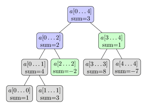
পদ্ধতিটি নিম্নলিখিত চিত্রে চিত্রিত হয়েছে। আবার অ্যারে $a = [1, 3, -2, 8, -7]$ ব্যবহার করা হয়, এবং এখানে আমরা যোগফল $\sum_{i=2}^4 a[i]$ গণনা করতে চাই। রঙিন ভার্টেক্সগুলি পরিদর্শন করা হবে, এবং আমরা সবুজ ভার্টেক্সগুলির পূর্বনির্ধারিত মানগুলি ব্যবহার করব। এটি আমাদের ফলাফল $-2 + 1 = -1$ দেয়।
কেন এই অ্যালগরিদমের কমপ্লেক্সিটি $O(\log n)$? এই কমপ্লেক্সিটি প্রদর্শন করতে আমরা ট্রির প্রতিটি স্তর দেখি। দেখা যায় যে প্রতিটি স্তরের জন্য আমরা চারটিরও বেশি ভার্টেক্স পরিদর্শন করি না। এবং যেহেতু ট্রির উচ্চতা $O(\log n)$, আমরা পছন্দসই চলমান সময় পাই।
আমরা এই প্রস্তাব (প্রতিটি স্তরে সর্বাধিক চারটি ভার্টেক্স) প্রমাণ করতে পারি ইন্ডাকশন দ্বারা। প্রথম স্তরে, আমরা শুধুমাত্র একটি ভার্টেক্স, রুট ভার্টেক্স পরিদর্শন করি, তাই এখানে আমরা চারটিরও কম ভার্টেক্স পরিদর্শন করি। এখন একটি স্বেচ্ছাচারী স্তর দেখি। ইন্ডাকশন হাইপোথিসিস দ্বারা, আমরা সর্বাধিক চারটি ভার্টেক্স পরিদর্শন করি। যদি আমরা সর্বাধিক দুটি ভার্টেক্স পরিদর্শন করি, পরবর্তী স্তরে সর্বাধিক চারটি ভার্টেক্স রয়েছে। এটি তুচ্ছ, কারণ প্রতিটি ভার্টেক্স সর্বাধিক দুটি রিকার্সিভ কল সৃষ্টি করতে পারে। তাই আসুন ধরুন যে আমরা বর্তমান স্তরে তিন বা চারটি ভার্টেক্স পরিদর্শন করি। সেই ভার্টেক্সগুলি থেকে, আমরা মধ্যের ভার্টেক্সগুলি আরও সাবধানে বিশ্লেষণ করব। যেহেতু সাম কোয়েরি একটি ক্রমাগত সাবঅ্যারের যোগফল জিজ্ঞাসা করে, আমরা জানি যে মধ্যের পরিদর্শিত ভার্টেক্সগুলির সাথে সম্পর্কিত সেগমেন্টগুলি সাম কোয়েরির সেগমেন্ট দ্বারা সম্পূর্ণভাবে কভার করা হবে। অতএব এই ভার্টেক্সগুলি কোনো রিকার্সিভ কল করবে না। তাই শুধুমাত্র সবচেয়ে বাম এবং সবচেয়ে ডান ভার্টেক্সের রিকার্সিভ কল করার সম্ভাবনা থাকবে। এবং সেগুলি শুধুমাত্র সর্বাধিক চারটি রিকার্সিভ কল সৃষ্টি করবে, তাই পরবর্তী স্তরও প্রস্তাব সন্তুষ্ট করবে। আমরা বলতে পারি যে একটি শাখা কোয়েরির বাম সীমানার কাছে পৌঁছায়, এবং দ্বিতীয় শাখা ডানটির কাছে পৌঁছায়।
অতএব আমরা মোট সর্বাধিক $4 \log n$ ভার্টেক্স পরিদর্শন করি, এবং এটি $O(\log n)$ এর একটি চলমান সময়ের সমান।
উপসংহারে কোয়েরিটি ইনপুট সেগমেন্টকে বেশ কয়েকটি সাব-সেগমেন্টে বিভক্ত করে কাজ করে যার জন্য সমস্ত যোগফল ইতিমধ্যে প্রি-কম্পিউটেড এবং ট্রিতে সংরক্ষিত। এবং যখনই কোয়েরি সেগমেন্ট ভার্টেক্স সেগমেন্টের সাথে মিলে যায় তখন যদি আমরা বিভাজন থামাই, তবে আমাদের শুধুমাত্র $O(\log n)$ এই ধরনের সেগমেন্ট প্রয়োজন, যা সেগমেন্ট ট্রির কার্যকারিতা দেয়।
আপডেট কোয়েরি#
এখন আমরা অ্যারেতে একটি নির্দিষ্ট উপাদান পরিবর্তন করতে চাই, ধরুন আমরা অ্যাসাইনমেন্ট $a[i] = x$ করতে চাই। এবং আমাদের সেগমেন্ট ট্রি পুনর্নির্মাণ করতে হবে, যাতে এটি নতুন, পরিবর্তিত অ্যারের সাথে মিল খায়।
এই কোয়েরি সাম কোয়েরির চেয়ে সহজ। সেগমেন্ট ট্রির প্রতিটি স্তর অ্যারের একটি বিভাজন গঠন করে। অতএব একটি উপাদান $a[i]$ প্রতিটি স্তর থেকে শুধুমাত্র একটি সেগমেন্টে অবদান রাখে। এইভাবে শুধুমাত্র $O(\log n)$ ভার্টেক্স আপডেট করা প্রয়োজন।
এটি সহজে দেখা যায় যে আপডেট অনুরোধটি একটি রিকার্সিভ ফাংশন ব্যবহার করে প্রয়োগ করা যেতে পারে। ফাংশনটি বর্তমান ট্রি ভার্টেক্স পাস করা হয়, এবং এটি দুটি চাইল্ড ভার্টেক্সের একটির সাথে নিজেকে রিকার্সিভভাবে কল করে (যেটি তার সেগমেন্টে $a[i]$ ধারণ করে), এবং এর পরে এর যোগফল মান পুনরায় গণনা করে, যেভাবে বিল্ড পদ্ধতিতে করা হয় (অর্থাৎ এর দুটি চাইল্ডের যোগফল হিসাবে)।
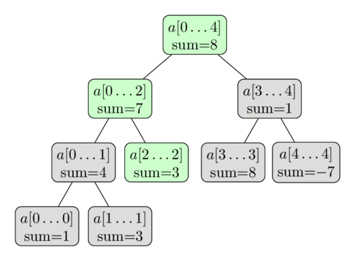
আবার এখানে একই অ্যারে ব্যবহার করে একটি ভিজ্যুয়ালাইজেশন রয়েছে। এখানে আমরা আপডেট $a[2] = 3$ সম্পাদন করি। সবুজ ভার্টেক্সগুলি হল সেই ভার্টেক্স যা আমরা পরিদর্শন এবং আপডেট করি।
ইমপ্লিমেন্টেশন#
প্রধান বিবেচনা হল সেগমেন্ট ট্রি কীভাবে সংরক্ষণ করা যায়। অবশ্যই আমরা একটি $\text{vertex}$ স্ট্রাক্ট সংজ্ঞায়িত করতে পারি এবং বস্তু তৈরি করতে পারি, যা সেগমেন্টের সীমানা, এর যোগফল এবং অতিরিক্তভাবে এর চাইল্ড ভার্টেক্সের পয়েন্টার সংরক্ষণ করে। তবে, এটি পয়েন্টার আকারে অনেক রিডানড্যান্ট তথ্য সংরক্ষণ করতে প্রয়োজন। আমরা একটি সরল কৌশল ব্যবহার করব এটি আরও দক্ষ করতে একটি ইমপ্লিসিট ডেটা স্ট্রাকচার ব্যবহার করে: শুধুমাত্র একটি অ্যারেতে যোগফল সংরক্ষণ করা। (একটি অনুরূপ পদ্ধতি বাইনারি হিপের জন্য ব্যবহার করা হয়)। সূচক १ এ রুট ভার্টেক্সের যোগফল, সূচক २ এবং ३ এ এর দুটি চাইল্ড ভার্টেক্সের যোগফল, সূচক ४ থেকে ७ এ সেই দুটি ভার্টেক্সের চাইল্ডদের যোগফল, এবং এভাবে চলে। १-ইন্ডেক্সিং সহ, সুবিধামত সূচক $i$ এ একটি ভার্টেক্সের বাম চাইল্ড সূচক $२i$ তে সংরক্ষিত হয়, এবং ডানটি সূচক $२i + १$ তে। সমানভাবে, সূচক $i$ এ একটি ভার্টেক্সের পিতামাতা $i/२$ তে সংরক্ষিত হয় (পূর্ণসংখ্যা বিভাগ)।
এটি ইমপ্লিমেন্টেশনকে অনেক সহজ করে। আমাদের স্মৃতিতে ট্রির কাঠামো সংরক্ষণ করতে হবে না। এটি অন্তর্নিহিতভাবে সংজ্ঞায়িত। আমাদের শুধুমাত্র একটি অ্যারে প্রয়োজন যা সমস্ত সেগমেন্টের যোগফল ধারণ করে।
আগে উল্লেখ করা হয়েছে, আমাদের সর্বাধিক $4n$ ভার্টেক্স সংরক্ষণ করতে হবে। এটি কম হতে পারে, তবে সুবিধার জন্য আমরা সর্বদা আকার $4n$ এর একটি অ্যারে বরাদ্দ করি। যোগফল অ্যারেতে এমন কিছু উপাদান থাকবে যা প্রকৃত ট্রিতে কোনো ভার্টেক্সের সাথে সম্পর্কিত নয়, তবে এটি ইমপ্লিমেন্টেশনকে জটিল করে না।
তাই আমরা সেগমেন্ট ট্রি সহজভাবে একটি অ্যারে $t[]$ হিসাবে ইনপুট আকার $n$ এর চারগুণ আকার সহ সংরক্ষণ করি:
int n, t[4*MAXN];একটি প্রদত্ত অ্যারে $a[]$ থেকে সেগমেন্ট ট্রি নির্মাণের পদ্ধতি এইরকম দেখায়: এটি প্যারামিটার $a[]$ (ইনপুট অ্যারে), $v$ (বর্তমান ভার্টেক্সের সূচক), এবং বর্তমান সেগমেন্টের সীমানা $tl$ এবং $tr$ সহ একটি রিকার্সিভ ফাংশন। প্রধান প্রোগ্রামে এই ফাংশনটি রুট ভার্টেক্সের প্যারামিটার সহ বলা হবে: $v = १$, $tl = ०$, এবং $tr = n - १$।
void build(int a[], int v, int tl, int tr) {
    if (tl == tr) {
        t[v] = a[tl];
    } else {
        int tm = (tl + tr) / 2;
        build(a, v*2, tl, tm);
        build(a, v*2+1, tm+1, tr);
        t[v] = t[v*2] + t[v*2+1];
    }
}
এর বাইরে সাম কোয়েরিতে উত্তর দেওয়ার ফাংশনটিও একটি রিকার্সিভ ফাংশন, যা বর্তমান ভার্টেক্স/সেগমেন্ট সম্পর্কিত তথ্য (অর্থাৎ সূচক $v$ এবং সীমানা $tl$ এবং $tr$) এবং কোয়েরির সীমানা সম্পর্কিত তথ্য $l$ এবং $r$ প্যারামিটার হিসাবে পায়। কোড সরল করার জন্য, এই ফাংশনটি সর্বদা দুটি রিকার্সিভ কল সম্পাদন করে, এমনকি যদি শুধুমাত্র একটি প্রয়োজন হয় - সেই ক্ষেত্রে অতিরিক্ত রিকার্সিভ কলটি $l > r$ হবে, এবং এটি ফাংশনের শুরুতে একটি অতিরিক্ত চেক ব্যবহার করে সহজেই ধরা যেতে পারে।
int sum(int v, int tl, int tr, int l, int r) {
    if (l > r)
        return 0;
    if (l == tl && r == tr) {
        return t[v];
    }
    int tm = (tl + tr) / 2;
    return sum(v*2, tl, tm, l, min(r, tm))
           + sum(v*2+1, tm+1, tr, max(l, tm+1), r);
}
অবশেষে আপডেট কোয়েরি। ফাংশনটি বর্তমান ভার্টেক্স/সেগমেন্ট সম্পর্কিত তথ্যও পাবে, এবং অতিরিক্তভাবে আপডেট কোয়েরির প্যারামিটার (অর্থাৎ উপাদানের অবস্থান এবং এর নতুন মান)।
void update(int v, int tl, int tr, int pos, int new_val) {
    if (tl == tr) {
        t[v] = new_val;
    } else {
        int tm = (tl + tr) / 2;
        if (pos <= tm)
            update(v*2, tl, tm, pos, new_val);
        else
            update(v*2+1, tm+1, tr, pos, new_val);
        t[v] = t[v*2] + t[v*2+1];
    }
}
মেমোরি সাশ্রয়ী ইমপ্লিমেন্টেশন#
বেশিরভাগ মানুষ পূর্ববর্তী বিভাগ থেকে ইমপ্লিমেন্টেশন ব্যবহার করে। যদি আপনি অ্যারে t তাকান আপনি দেখতে পারবেন যে এটি একটি BFS ট্রাভার্সাল (স্তর-অর্ডার ট্রাভার্সাল) এর ক্রমে ট্রি নোডের নাম্বারিং অনুসরণ করে।
এই ট্রাভার্সাল ব্যবহার করে ভার্টেক্স $v$ এর চাইল্ডগুলি যথাক্রমে $२v$ এবং $२v + १$ হয়।
তবে যদি $n$ দুইয়ের শক্তি না হয়, এই পদ্ধতিটি কিছু সূচক এড়িয়ে যাবে এবং অ্যারে t এর কিছু অংশ অব্যবহৃত রেখে যাবে।
মেমোরি খরচ $4n$ দ্বারা সীমিত, যদিও $n$ উপাদানের একটি অ্যারের সেগমেন্ট ট্রির জন্য শুধুমাত্র $२n - १$ ভার্টেক্স প্রয়োজন।
তবে এটি হ্রাস করা যায়। আমরা একটি Euler ট্যুর ট্রাভার্সাল (প্রি-অর্ডার ট্রাভার্সাল) এর ক্রমে ট্রির ভার্টেক্সগুলির নাম্বার পুনর্নির্ধারণ করি, এবং আমরা এই সমস্ত ভার্টেক্সগুলি একসাথে লিখি।
সূচক $v$ তে একটি ভার্টেক্স বিবেচনা করি, এবং এটি সেগমেন্ট $[l, r]$ এর জন্য দায়বদ্ধ, এবং $mid = \dfrac{l + r}{२}$। এটি স্পষ্ট যে বাম চাইল্ড সূচক $v + १$ থাকবে। বাম চাইল্ড সেগমেন্ট $[l, mid]$ এর জন্য দায়বদ্ধ, অর্থাৎ মোট বাম চাইল্ডের সাবট্রিতে $२ * (mid - l + १) - १$ ভার্টেক্স থাকবে। এইভাবে আমরা $v$ এর ডান চাইল্ডের সূচক গণনা করতে পারি। সূচকটি হবে $v + २ * (mid - l + १)$। এই নাম্বারিং দ্বারা আমরা প্রয়োজনীয় মেমোরি $२n$ এ হ্রাস অর্জন করি।
সেগমেন্ট ট্রির উন্নত সংস্করণ#
একটি সেগমেন্ট ট্রি একটি অত্যন্ত নমনীয় ডেটা স্ট্রাকচার, এবং অনেক বিভিন্ন দিক থেকে ভেরিয়েশন এবং এক্সটেনশন অনুমোদন করে। আসুন নীচের তাদের শ্রেণীবদ্ধ করার চেষ্টা করি।
আরও জটিল কোয়েরি#
সেগমেন্ট ট্রিকে একটি দিকে পরিবর্তন করা বেশ সহজ হতে পারে, যাতে এটি বিভিন্ন কোয়েরি গণনা করে (উদাহরণস্বরূপ সাম না করে ন্যূনতম / সর্বাধিক গণনা করা), তবে এটিও অত্যন্ত তুচ্ছ হতে পারে।
সর্বাধিক খুঁজে পাওয়া#
আমরা উপরে বর্ণিত সমস্যার অবস্থা সামান্য পরিবর্তন করি: যোগফল কোয়েরি করার পরিবর্তে, আমরা এখন সর্বাধিক কোয়েরি করব।
ট্রিটি উপরে বর্ণিত ট্রির সঠিক একই কাঠামো থাকবে। আমাদের শুধুমাত্র $\text{build}$ এবং $\text{update}$ ফাংশনে $t[v]$ কীভাবে গণনা করা হয় তা পরিবর্তন করতে হবে। $t[v]$ এখন সম্পর্কিত সেগমেন্টের সর্বাধিক সংরক্ষণ করবে। এবং আমাদের $\text{sum}$ ফাংশনের রিটার্ন মানের গণনাও পরিবর্তন করতে হবে (সর্বাধিক দ্বারা যোগফল প্রতিস্থাপন করা)।
অবশ্যই এই সমস্যাটি সর্বাধিক না করে ন্যূনতম গণনা করার জন্য সহজেই পরিবর্তন করা যেতে পারে।
এই সমস্যার একটি ইমপ্লিমেন্টেশন দেখানোর পরিবর্তে, পরবর্তী বিভাগে এই সমস্যার একটি আরও জটিল সংস্করণের জন্য ইমপ্লিমেন্টেশন দেওয়া হবে।
সর্বাধিক এবং এটি যতবার প্রদর্শিত হয় তার সংখ্যা খুঁজে পাওয়া#
এই কাজটি পূর্ববর্তী একটির সাথে অনুরূপ। সর্বাধিক খুঁজে পাওয়া ছাড়াও, আমাদের সর্বাধিকের সংখ্যাও খুঁজে পেতে হবে।
এই সমস্যা সমাধানের জন্য, আমরা ট্রিতে প্রতিটি ভার্টেক্সে একটি সংখ্যার জোড়া সংরক্ষণ করি: সর্বাধিক ছাড়াও আমরা সম্পর্কিত সেগমেন্টে এটির সংখ্যাও সংরক্ষণ করি। $t[v]$ তে সংরক্ষণ করার জন্য সঠিক জোড়া নির্ধারণ করা এখনও চাইল্ড ভার্টেক্সে সংরক্ষিত জোড়ার তথ্য ব্যবহার করে ধ্রুবক সময়ে করা যায়। এই ধরনের দুটি জোড়া একটি আলাদা ফাংশনে একত্রিত করা উচিত, কারণ এটি এমন একটি অপারেশন যা আমরা ট্রি তৈরি করার সময়, সর্বাধিক কোয়েরিতে উত্তর দেওয়ার সময় এবং পরিবর্তন সম্পাদনের সময় করব।
pair<int, int> t[4*MAXN];

pair<int, int> combine(pair<int, int> a, pair<int, int> b) {
    if (a.first > b.first)
        return a;
    if (b.first > a.first)
        return b;
    return make_pair(a.first, a.second + b.second);
}

void build(int a[], int v, int tl, int tr) {
    if (tl == tr) {
        t[v] = make_pair(a[tl], 1);
    } else {
        int tm = (tl + tr) / 2;
        build(a, v*2, tl, tm);
        build(a, v*2+1, tm+1, tr);
        t[v] = combine(t[v*2], t[v*2+1]);
    }
}

pair<int, int> get_max(int v, int tl, int tr, int l, int r) {
    if (l > r)
        return make_pair(-INF, 0);
    if (l == tl && r == tr)
        return t[v];
    int tm = (tl + tr) / 2;
    return combine(get_max(v*2, tl, tm, l, min(r, tm)),
                   get_max(v*2+1, tm+1, tr, max(l, tm+1), r));
}

void update(int v, int tl, int tr, int pos, int new_val) {
    if (tl == tr) {
        t[v] = make_pair(new_val, 1);
    } else {
        int tm = (tl + tr) / 2;
        if (pos <= tm)
            update(v*2, tl, tm, pos, new_val);
        else
            update(v*2+1, tm+1, tr, pos, new_val);
        t[v] = combine(t[v*2], t[v*2+1]);
    }
}
সর্বশ্রেষ্ঠ সাধারণ ভাজক / ন্যূনতম সাধারণ গুণিতক গণনা করা#
এই সমস্যায় আমরা অ্যারের প্রদত্ত রেঞ্জের সমস্ত সংখ্যার GCD / LCM গণনা করতে চাই।
সেগমেন্ট ট্রির এই আকর্ষণীয় ভেরিয়েশনটি ঠিক একইভাবে সমাধান করা যায় যেমনিতে আমরা সাম / ন্যূনতম / সর্বাধিক কোয়েরির জন্য সেগমেন্ট ট্রি তৈরি করেছি: ট্রির প্রতিটি ভার্টেক্সে সম্পর্কিত ভার্টেক্সের GCD / LCM সংরক্ষণ করা যথেষ্ট। দুটি ভার্টেক্স একত্রিত করা উভয় ভার্টেক্সের GCD / LCM গণনা করে করা যেতে পারে।
শূন্যের সংখ্যা গণনা করা, $k$-তম শূন্য অনুসন্ধান করা#
এই সমস্যায় আমরা একটি প্রদত্ত রেঞ্জে শূন্যের সংখ্যা খুঁজে পেতে চাই, এবং অতিরিক্তভাবে একটি দ্বিতীয় ফাংশন ব্যবহার করে $k$-তম শূন্যের সূচক খুঁজে পেতে চাই।
আবার আমাদের ট্রির সংরক্ষিত মানগুলি কিছুটা পরিবর্তন করতে হবে: এবার আমরা $t[]$ তে প্রতিটি সেগমেন্টে শূন্যের সংখ্যা সংরক্ষণ করব। এটি পরিষ্কার যে $\text{build}$, $\text{update}$ এবং $\text{count\_zeros}$ ফাংশন কীভাবে প্রয়োগ করতে হয়, আমরা সরলভাবে সাম কোয়েরি সমস্যা থেকে ধারণা ব্যবহার করতে পারি। এইভাবে আমরা সমস্যার প্রথম অংশ সমাধান করেছি।
এখন আমরা অ্যারে $a[]$ তে $k$-তম শূন্য খুঁজে পাওয়ার সমস্যা সমাধান করতে শিখি। এই কাজ করার জন্য, আমরা সেগমেন্ট ট্রি নেমে আসব, রুট ভার্টেক্স থেকে শুরু করে, এবং প্রতিবার বাম বা ডান চাইল্ডে যাই, কোন সেগমেন্টে $k$-তম শূন্য আছে তার উপর নির্ভর করে। কোন চাইল্ডে যেতে হবে তা সিদ্ধান্ত নিতে, বাম ভার্টেক্সের সাথে সম্পর্কিত সেগমেন্টে প্রদর্শিত শূন্যের সংখ্যা দেখা যথেষ্ট। যদি এই পূর্বনির্ধারিত গণনা $k$ এর চেয়ে বড় বা সমান হয়, তবে বাম চাইল্ডে নেমে যাওয়া প্রয়োজন, অন্যথায় ডান চাইল্ডে নেমে যান। লক্ষ্য করুন, যদি আমরা ডান চাইল্ড বেছে নিই, আমাদের $k$ থেকে বাম চাইল্ডের শূন্যের সংখ্যা বিয়োগ করতে হবে।
ইমপ্লিমেন্টেশনে আমরা বিশেষ ক্ষেত্র হ্যান্ডল করতে পারি, $a[]$ -১ ফেরত দিয়ে $k$ এর চেয়ে কম শূন্য থাকলে।
int find_kth(int v, int tl, int tr, int k) {
    if (k > t[v])
        return -1;
    if (tl == tr)
        return tl;
    int tm = (tl + tr) / 2;
    if (t[v*2] >= k)
        return find_kth(v*2, tl, tm, k);
    else
        return find_kth(v*2+1, tm+1, tr, k - t[v*2]);
}
দেওয়া পরিমাণ সহ অ্যারে প্রিফিক্স অনুসন্ধান করা#
কাজটি নিম্নরূপ: একটি প্রদত্ত মান $x$ এর জন্য আমাদের দ্রুত সবচেয়ে ছোট সূচক $i$ খুঁজে পেতে হবে যাতে অ্যারে $a[]$ এর প্রথম $i$ উপাদানের যোগফল $x$ এর চেয়ে বড় বা সমান হয় (ধরে নিয়ে যে অ্যারে $a[]$ শুধুমাত্র অ-নেতিবাচক মান ধারণ করে)।
এই কাজটি সেগমেন্ট ট্রির সাথে প্রিফিক্সের যোগফল গণনা করে বাইনারি অনুসন্ধান ব্যবহার করে সমাধান করা যায়। তবে এটি $O(\log^2 n)$ সমাধানে নিয়ে যাবে।
পরিবর্তে আমরা পূর্ববর্তী বিভাগের একই ধারণা ব্যবহার করতে পারি, এবং ট্রি নেমে আসার মাধ্যমে অবস্থান খুঁজে পেতে পারি: বাম চাইল্ডের যোগফলের উপর নির্ভর করে প্রতিবার বাম বা ডানে যাই। এইভাবে $O(\log n)$ সময়ে উত্তর খুঁজে পাই।
একটি প্রদত্ত পরিমাণের চেয়ে বড় প্রথম উপাদান অনুসন্ধান করা#
কাজটি নিম্নরূপ: একটি প্রদত্ত মান $x$ এবং রেঞ্জ $a[l \dots r]$ এর জন্য রেঞ্জ $a[l \dots r]$ তে সবচেয়ে ছোট $i$ খুঁজে পাই, যাতে $a[i]$ $x$ এর চেয়ে বড় হয়।
এই কাজটি সেগমেন্ট ট্রির সাথে সর্বাধিক প্রিফিক্স কোয়েরির উপর বাইনারি অনুসন্ধান ব্যবহার করে সমাধান করা যায়। তবে, এটি $O(\log^2 n)$ সমাধানে নিয়ে যাবে।
পরিবর্তে, আমরা পূর্ববর্তী বিভাগের একই ধারণা ব্যবহার করতে পারি, এবং ট্রি নেমে আসার মাধ্যমে অবস্থান খুঁজে পেতে পারি: বাম চাইল্ডের সর্বাধিক মানের উপর নির্ভর করে প্রতিবার বাম বা ডানে যাই। এইভাবে $O(\log n)$ সময়ে উত্তর খুঁজে পাই।
int get_first(int v, int tl, int tr, int l, int r, int x) {
    if(tl > r || tr < l) return -1;
    if(t[v] <= x) return -1;

    if (tl== tr) return tl;

    int tm = tl + (tr-tl)/2;
    int left = get_first(2*v, tl, tm, l, r, x);
    if(left != -1) return left;
    return get_first(2*v+1, tm+1, tr, l ,r, x);
}
সর্বাধিক যোগফল সহ সাবসেগমেন্ট খুঁজে পাওয়া#
এখানে আবার প্রতিটি কোয়েরির জন্য একটি রেঞ্জ $a[l \dots r]$ পাই, এবার আমাদের একটি সাবসেগমেন্ট $a[l^\prime \dots r^\prime]$ খুঁজে পেতে হবে যাতে $l \le l^\prime$ এবং $r^\prime \le r$ এবং এই সেগমেন্টের উপাদানগুলির যোগফল সর্বাধিক হয়। আগে যেমন আমরা অ্যারের স্বতন্ত্র উপাদান পরিবর্তন করতে চাই। অ্যারের উপাদানগুলি ঋণাত্মক হতে পারে, এবং সর্বোত্তম সাবসেগমেন্ট খালি হতে পারে (উদাহরণস্বরূপ যদি সমস্ত উপাদান ঋণাত্মক হয়)।
এই সমস্যাটি সেগমেন্ট ট্রির একটি অ-তুচ্ছ ব্যবহার। এবার আমরা প্রতিটি ভার্টেক্সের জন্য চারটি মান সংরক্ষণ করব: সেগমেন্টের যোগফল, সর্বাধিক প্রিফিক্স যোগফল, সর্বাধিক সাফিক্স যোগফল, এবং এটিতে সর্বাধিক সাবসেগমেন্টের যোগফল। অন্য কথায় সেগমেন্ট ট্রির প্রতিটি সেগমেন্টের জন্য উত্তর ইতিমধ্যে পূর্বনির্ধারিত যেমন সেগমেন্টের বাম এবং ডান সীমানা স্পর্শকারী সেগমেন্টের উত্তরগুলি।
এই ধরনের ডেটা সহ একটি ট্রি তৈরি করতে কীভাবে? আবার আমরা এটি একটি রিকার্সিভ উপায়ে গণনা করি: আমরা প্রথমে বাম এবং ডান চাইল্ডের জন্য সমস্ত চারটি মান গণনা করি, এবং তারপর বর্তমান ভার্টেক্সের চারটি মান সংরক্ষণ করতে সেগুলি একত্রিত করি। বর্তমান ভার্টেক্সের উত্তর নিম্নোক্তগুলির মধ্যে যেকোনো একটি:
- বাম চাইল্ডের উত্তর, যার অর্থ সর্বোত্তম সাবসেগমেন্ট সম্পূর্ণভাবে বাম চাইল্ডের সেগমেন্টে রাখা
- ডান চাইল্ডের উত্তর, যার অর্থ সর্বোত্তম সাবসেগমেন্ট সম্পূর্ণভাবে ডান চাইল্ডের সেগমেন্টে রাখা
- বাম চাইল্ডের সর্বাধিক সাফিক্স যোগফল এবং ডান চাইল্ডের সর্বাধিক প্রিফিক্স যোগফলের যোগফল, যার অর্থ সর্বোত্তম সাবসেগমেন্ট উভয় চাইল্ডের সাথে ছেদ করে।
সুতরাং বর্তমান ভার্টেক্সের উত্তর এই তিনটি মানের সর্বাধিক। সর্বাধিক প্রিফিক্স / সাফিক্স যোগফল গণনা আরও সহজ। এখানে $\text{merge}$ ফাংশনের ইমপ্লিমেন্টেশন রয়েছে, যা শুধুমাত্র বাম এবং ডান চাইল্ড থেকে ডেটা পায়, এবং বর্তমান ভার্টেক্সের ডেটা রিটার্ন করে।
struct data {
    int sum, pref, suff, ans;
};

data combine(data l, data r) {
    data res;
    res.sum = l.sum + r.sum;
    res.pref = max(l.pref, l.sum + r.pref);
    res.suff = max(r.suff, r.sum + l.suff);
    res.ans = max(max(l.ans, r.ans), l.suff + r.pref);
    return res;
}
$\text{merge}$ ফাংশন ব্যবহার করে সেগমেন্ট ট্রি তৈরি করা সহজ। আমরা এটি পূর্ববর্তী ইমপ্লিমেন্টেশনের মতোই প্রয়োগ করতে পারি। লিফ ভার্টেক্স শুরু করতে, আমরা অতিরিক্তভাবে সহায়ক ফাংশন $\text{make\_data}$ তৈরি করি, যা একটি একক মান সম্পর্কিত তথ্য ধারণ করে এমন একটি $\text{data}$ অবজেক্ট রিটার্ন করবে।
data make_data(int val) {
    data res;
    res.sum = val;
    res.pref = res.suff = res.ans = max(0, val);
    return res;
}

void build(int a[], int v, int tl, int tr) {
    if (tl == tr) {
        t[v] = make_data(a[tl]);
    } else {
        int tm = (tl + tr) / 2;
        build(a, v*2, tl, tm);
        build(a, v*2+1, tm+1, tr);
        t[v] = combine(t[v*2], t[v*2+1]);
    }
}

void update(int v, int tl, int tr, int pos, int new_val) {
    if (tl == tr) {
        t[v] = make_data(new_val);
    } else {
        int tm = (tl + tr) / 2;
        if (pos <= tm)
            update(v*2, tl, tm, pos, new_val);
        else
            update(v*2+1, tm+1, tr, pos, new_val);
        t[v] = combine(t[v*2], t[v*2+1]);
    }
}
কোয়েরির উত্তর কিভাবে গণনা করতে হয় তা অবশেষ। এর উত্তর দিতে, আমরা আগের মতো ট্রি নেমে যাই, কোয়েরিকে বেশ কয়েকটি সাবসেগমেন্টে বিভক্ত করি যা সেগমেন্ট ট্রির সেগমেন্টের সাথে মিল খায়, এবং তাদের উত্তরগুলি একটি একক উত্তরে একত্রিত করি কোয়েরির জন্য। তারপর এটি স্পষ্ট হওয়া উচিত যে কাজটি সাধারণ সেগমেন্ট ট্রির মতোই, তবে মানগুলি যোগ করা / ন্যূনতম / সর্বাধিক করার পরিবর্তে, আমরা $\text{merge}$ ফাংশন ব্যবহার করি।
data query(int v, int tl, int tr, int l, int r) {
    if (l > r)
        return make_data(0);
    if (l == tl && r == tr)
        return t[v];
    int tm = (tl + tr) / 2;
    return combine(query(v*2, tl, tm, l, min(r, tm)),
                   query(v*2+1, tm+1, tr, max(l, tm+1), r));
}
প্রতিটি ভার্টেক্সে সম্পূর্ণ সাবঅ্যারে সংরক্ষণ করা#
এটি একটি আলাদা সাবসেকশন যা অন্যদের থেকে আলাদা হয়ে দাঁড়িয়ে আছে, কারণ সেগমেন্ট ট্রির প্রতিটি ভার্টেক্সে আমরা সম্পর্কিত সেগমেন্ট সম্পর্কিত তথ্য সংক্ষিপ্ত ফর্মে (যোগফল, ন্যূনতম, সর্বাধিক, …) সংরক্ষণ করি না, বরং সেগমেন্টের সমস্ত উপাদান সংরক্ষণ করি। এইভাবে সেগমেন্ট ট্রির মূল অ্যারের সমস্ত উপাদান সংরক্ষণ করবে, বাম চাইল্ড ভার্টেক্স অ্যারের প্রথম অর্ধ সংরক্ষণ করবে, ডান ভার্টেক্স দ্বিতীয় অর্ধ, এবং এভাবে চলে।
এই প্রযুক্তির সবচেয়ে সাধারণ প্রয়োগে আমরা উপাদানগুলি সাজানো ক্রমে সংরক্ষণ করি। আরও জটিল সংস্করণে উপাদানগুলি তালিকায় সংরক্ষিত হয় না, বরং আরও উন্নত ডেটা স্ট্রাকচার (সেট, ম্যাপ, …)। তবে এই সমস্ত পদ্ধতির সাধারণ ফ্যাক্টর রয়েছে যে প্রতিটি ভার্টেক্স রৈখিক মেমোরি প্রয়োজন (অর্থাৎ সম্পর্কিত সেগমেন্টের দৈর্ঘ্যের সাথে সমানুপাতিক)।
এই সেগমেন্ট ট্রি বিবেচনার সময় প্রথম প্রাকৃতিক প্রশ্ন হল মেমোরি খরচ সম্পর্কে। স্বজ্ঞাতভাবে এটি $O(n^२)$ মেমোরির মতো দেখতে পারে, তবে দেখা যায় যে সম্পূর্ণ ট্রি শুধুমাত্র $O(n \log n)$ মেমোরির প্রয়োজন। কেন এটি এমন? অত্যন্ত সহজভাবে, কারণ অ্যারের প্রতিটি উপাদান $O(\log n)$ সেগমেন্টে পড়ে (মনে রাখবেন ট্রির উচ্চতা $O(\log n)$)।
তাই এই ধরনের সেগমেন্ট ট্রির স্পষ্ট বিলাসিতা সত্ত্বেও, এটি সাধারণ সেগমেন্ট ট্রির চেয়ে সামান্য বেশি মেমোরি ব্যবহার করে।
এই ডেটা স্ট্রাকচারের বেশ কয়েকটি সাধারণ অ্যাপ্লিকেশন নিচে বর্ণিত। এই সেগমেন্ট ট্রিগুলির २D ডেটা স্ট্রাকচারের সাথে সাদৃশ্য লক্ষ্য করা মূল্যবান (প্রকৃতপক্ষে এটি একটি २D ডেটা স্ট্রাকচার, তবে বরং সীমিত ক্ষমতা সহ)।
নির্দিষ্ট সংখ্যার চেয়ে বড় বা সমান ক্ষুদ্রতম সংখ্যা খুঁজুন। কোনো পরিবর্তন কোয়েরি নেই।#
আমরা নিম্নোক্ত ফর্মের কোয়েরির উত্তর দিতে চাই: তিনটি প্রদত্ত সংখ্যার জন্য $(l, r, x)$ আমাদের সেগমেন্ট $a[l \dots r]$ তে ন্যূনতম সংখ্যা খুঁজে পেতে হবে যা $x$ এর চেয়ে বড় বা সমান।
আমরা একটি সেগমেন্ট ট्रি তৈরি করি। প্রতিটি ভার্টেক্সে আমরা সম্পর্কিত সেগমেন্টে ঘটে এমন সমস্ত সংখ্যার একটি সাজানো তালিকা সংরক্ষণ করি, উপরে বর্ণিত হিসাবে। এই ধরনের সেগমেন্ট ট्रি যতটা সম্ভব কার্যকরভাবে তৈরি করতে কীভাবে? সর্বদার মতো আমরা এই সমস্যাটি রিকার্সিভভাবে পদ্ধতি করি: বাম এবং ডান চাইল্ডের তালিকাগুলি ইতিমধ্যে নির্মিত, এবং আমরা বর্তমান ভার্টেক্সের জন্য তালিকা তৈরি করতে চাই। এই দৃষ্টিকোণ থেকে অপারেশন এখন তুচ্ছ এবং রৈখিক সময়ে সম্পাদিত হতে পারে: আমাদের শুধুমাত্র দুটি সাজানো তালিকা একটিতে একত্রিত করতে হবে, যা দুটি পয়েন্টার ব্যবহার করে তাদের উপর পুনরাবৃত্তি করে করা যায়। C++ STL ইতিমধ্যে এই অ্যালগরিদমের একটি ইমপ্লিমেন্টেশন রয়েছে।
সেগমেন্ট ট्রির এই কাঠামো এবং মার্জ সর্ট অ্যালগরিদমের সাথে সাদৃশ্যের কারণে, ডেটা স্ট্রাকচারকে প্রায়ই “মার্জ সর্ট ট्রি” বলা হয়।
vector<int> t[4*MAXN];

void build(int a[], int v, int tl, int tr) {
    if (tl == tr) {
        t[v] = vector<int>(1, a[tl]);
    } else {
        int tm = (tl + tr) / 2;
        build(a, v*2, tl, tm);
        build(a, v*2+1, tm+1, tr);
        merge(t[v*2].begin(), t[v*2].end(), t[v*2+1].begin(), t[v*2+1].end(),
              back_inserter(t[v]));
    }
}
আমরা ইতিমধ্যে জানি যে এইভাবে নির্মিত সেগমেন্ট ট्রি $O(n \log n)$ মেমোরির প্রয়োজন। এবং এই ইমপ্লিমেন্টেশনের জন্য ধন্যবাদ এর নির্মাণও $O(n \log n)$ সময় নেয়, সর্বশেষ প্রতিটি তালিকা এর আকারের সাপেক্ষে রৈখিক সময়ে নির্মিত হয়।
এখন কোয়েরির উত্তর বিবেচনা করুন। আমরা ট্রি নেমে যাব, সাধারণ সেগমেন্ট ট्রির মতো, আমাদের সেগমেন্ট $a[l \dots r]$ কে বেশ কয়েকটি সাবসেগমেন্টে বিভক্ত করি (সর্বাধিক $O(\log n)$ টুকরায়)। এটি স্পষ্ট যে সম্পূর্ণ উত্তর প্রতিটি সাবকোয়েরির ন্যূনতম। তাই এখন আমাদের শুধুমাত্র বুঝতে হবে, ট্রির কিছু ভার্টেক্সের সাথে সামঞ্জস্যপূর্ণ এই ধরনের একটি সাবসেগমেন্টে কোয়েরির উত্তর কীভাবে দেওয়া যায়।
আমরা সেগমেন্ট ট्রির কোনো ভার্টেক্সে রয়েছি এবং কোয়েরির উত্তর গণনা করতে চাই, অর্থাৎ একটি প্রদত্ত সংখ্যা $x$ এর চেয়ে বড় বা সমান ন্যূনতম সংখ্যা খুঁজুন। যেহেতু ভার্টেক্সে উপাদানের তালিকা সাজানো ক্রমে রয়েছে, আমরা সহজভাবে এই তালিকায় একটি বাইনারি অনুসন্ধান সম্পাদন করতে এবং $x$ এর চেয়ে বড় বা সমান প্রথম সংখ্যা রিটার্ন করতে পারি।
এইভাবে ট্রির একটি সেগমেন্টে কোয়েরির উত্তর $O(\log n)$ সময় নেয়, এবং সম্পূর্ণ কোয়েরি $O(\log^२ n)$ এ প্রক্রিয়া করা হয়।
int query(int v, int tl, int tr, int l, int r, int x) {
    if (l > r)
        return INF;
    if (l == tl && r == tr) {
        vector<int>::iterator pos = lower_bound(t[v].begin(), t[v].end(), x);
        if (pos != t[v].end())
            return *pos;
        return INF;
    }
    int tm = (tl + tr) / 2;
    return min(query(v*2, tl, tm, l, min(r, tm), x),
               query(v*2+1, tm+1, tr, max(l, tm+1), r, x));
}
ধ্রুবক $\text{INF}$ অ্যারেতে সমস্ত সংখ্যার চেয়ে বড় কিছু বড় সংখ্যার সমান। এর ব্যবহার মানে সেগমেন্টে $x$ এর চেয়ে বড় বা সমান কোনো সংখ্যা নেই। এটির অর্থ “প্রদত্ত ইন্টারভালে কোনো উত্তর নেই”।
Find the smallest number greater or equal to a specified number. With modification queries.#
This task is similar to the previous. The last approach has a disadvantage, it was not possible to modify the array between answering queries. Now we want to do exactly this: a modification query will do the assignment $a[i] = y$.
The solution is similar to the solution of the previous problem, but instead of lists at each vertex of the Segment Tree, we will store a balanced list that allows you to quickly search for numbers, delete numbers, and insert new numbers. Since the array can contain a number repeated, the optimal choice is the data structure $\text{multiset}$.
The construction of such a Segment Tree is done in pretty much the same way as in the previous problem, only now we need to combine $\text{multiset}$s and not sorted lists. This leads to a construction time of $O(n \log^2 n)$ (in general merging two red-black trees can be done in linear time, but the C++ STL doesn’t guarantee this time complexity).
The $\text{query}$ function is also almost equivalent, only now the $\text{lower_bound}$ function of the $\text{multiset}$ function should be called instead ($\text{std::lower_bound}$ only works in $O(\log n)$ time if used with random-access iterators).
Finally the modification request. To process it, we must go down the tree, and modify all $\text{multiset}$ from the corresponding segments that contain the affected element. We simply delete the old value of this element (but only one occurrence), and insert the new value.
void update(int v, int tl, int tr, int pos, int new_val) {
    t[v].erase(t[v].find(a[pos]));
    t[v].insert(new_val);
    if (tl != tr) {
        int tm = (tl + tr) / 2;
        if (pos <= tm)
            update(v*2, tl, tm, pos, new_val);
        else
            update(v*2+1, tm+1, tr, pos, new_val);
    } else {
        a[pos] = new_val;
    }
}
Processing of this modification query also takes $O(\log^2 n)$ time.
Find the smallest number greater or equal to a specified number. Acceleration with “fractional cascading”.#
We have the same problem statement, we want to find the minimal number greater than or equal to $x$ in a segment, but this time in $O(\log n)$ time. We will improve the time complexity using the technique “fractional cascading”.
Fractional cascading is a simple technique that allows you to improve the running time of multiple binary searches, which are conducted at the same time. Our previous approach to the search query was, that we divide the task into several subtasks, each of which is solved with a binary search. Fractional cascading allows you to replace all of these binary searches with a single one.
The simplest and most obvious example of fractional cascading is the following problem: there are $k$ sorted lists of numbers, and we must find in each list the first number greater than or equal to the given number.
Instead of performing a binary search for each list, we could merge all lists into one big sorted list. Additionally for each element $y$ we store a list of results of searching for $y$ in each of the $k$ lists. Therefore if we want to find the smallest number greater than or equal to $x$, we just need to perform one single binary search, and from the list of indices we can determine the smallest number in each list. This approach however requires $O(n \cdot k)$ ($n$ is the length of the combined lists), which can be quite inefficient.
Fractional cascading reduces this memory complexity to $O(n)$ memory, by creating from the $k$ input lists $k$ new lists, in which each list contains the corresponding list and additionally also every second element of the following new list. Using this structure it is only necessary to store two indices, the index of the element in the original list, and the index of the element in the following new list. So this approach only uses $O(n)$ memory, and still can answer the queries using a single binary search.
But for our application we do not need the full power of fractional cascading. In our Segment Tree a vertex will contain the sorted list of all elements that occur in either the left or the right subtrees (like in the Merge Sort Tree). Additionally to this sorted list, we store two positions for each element. For an element $y$ we store the smallest index $i$, such that the $i$th element in the sorted list of the left child is greater or equal to $y$. And we store the smallest index $j$, such that the $j$th element in the sorted list of the right child is greater or equal to $y$. These values can be computed in parallel to the merging step when we build the tree.
How does this speed up the queries?
Remember, in the normal solution we did a binary search in every node. But with this modification, we can avoid all except one.
To answer a query, we simply do a binary search in the root node. This gives us the smallest element $y \ge x$ in the complete array, but it also gives us two positions. The index of the smallest element greater or equal $x$ in the left subtree, and the index of the smallest element $y$ in the right subtree. Notice that $\ge y$ is the same as $\ge x$, since our array doesn’t contain any elements between $x$ and $y$. In the normal Merge Sort Tree solution we would compute these indices via binary search, but with the help of the precomputed values we can just look them up in $O(1)$. And we can repeat that until we visited all nodes that cover our query interval.
To summarize, as usual we touch $O(\log n)$ nodes during a query. In the root node we do a binary search, and in all other nodes we only do constant work. This means the complexity for answering a query is $O(\log n)$.
But notice, that this uses three times more memory than a normal Merge Sort Tree, which already uses a lot of memory ($O(n \log n)$).
It is straightforward to apply this technique to a problem, that doesn’t require any modification queries. The two positions are just integers and can easily be computed by counting when merging the two sorted sequences.
It is still possible to also allow modification queries, but that complicates the entire code.
Instead of integers, you need to store the sorted array as multiset, and instead of indices you need to store iterators.
And you need to work very carefully, so that you increment or decrement the correct iterators during a modification query.
Other possible variations#
This technique implies a whole new class of possible applications. Instead of storing a $\text{vector}$ or a $\text{multiset}$ in each vertex, other data structures can be used: other Segment Trees (somewhat discussed in Generalization to higher dimensions), Fenwick Trees, Cartesian trees, etc.
Range updates (Lazy Propagation)#
All problems in the above sections discussed modification queries that only affected a single element of the array each. However the Segment Tree allows applying modification queries to an entire segment of contiguous elements, and perform the query in the same time $O(\log n)$.
Addition on segments#
We begin by considering problems of the simplest form: the modification query should add a number $x$ to all numbers in the segment $a[l \dots r]$. The second query, that we are supposed to answer, asked simply for the value of $a[i]$.
To make the addition query efficient, we store at each vertex in the Segment Tree how many we should add to all numbers in the corresponding segment. For example, if the query “add 3 to the whole array $a[0 \dots n-1]$” comes, then we place the number 3 in the root of the tree. In general we have to place this number to multiple segments, which form a partition of the query segment. Thus we don’t have to change all $O(n)$ values, but only $O(\log n)$ many.
If now there comes a query that asks the current value of a particular array entry, it is enough to go down the tree and add up all values found along the way.
void build(int a[], int v, int tl, int tr) {
    if (tl == tr) {
        t[v] = a[tl];
    } else {
        int tm = (tl + tr) / 2;
        build(a, v*2, tl, tm);
        build(a, v*2+1, tm+1, tr);
        t[v] = 0;
    }
}

void update(int v, int tl, int tr, int l, int r, int add) {
    if (l > r)
        return;
    if (l == tl && r == tr) {
        t[v] += add;
    } else {
        int tm = (tl + tr) / 2;
        update(v*2, tl, tm, l, min(r, tm), add);
        update(v*2+1, tm+1, tr, max(l, tm+1), r, add);
    }
}

int get(int v, int tl, int tr, int pos) {
    if (tl == tr)
        return t[v];
    int tm = (tl + tr) / 2;
    if (pos <= tm)
        return t[v] + get(v*2, tl, tm, pos);
    else
        return t[v] + get(v*2+1, tm+1, tr, pos);
}
Assignment on segments#
Suppose now that the modification query asks to assign each element of a certain segment $a[l \dots r]$ to some value $p$. As a second query we will again consider reading the value of the array $a[i]$.
To perform this modification query on a whole segment, you have to store at each vertex of the Segment Tree whether the corresponding segment is covered entirely with the same value or not. This allows us to make a “lazy” update: instead of changing all segments in the tree that cover the query segment, we only change some, and leave others unchanged. A marked vertex will mean, that every element of the corresponding segment is assigned to that value, and actually also the complete subtree should only contain this value. In a sense we are lazy and delay writing the new value to all those vertices. We can do this tedious task later, if this is necessary.
So after the modification query is executed, some parts of the tree become irrelevant - some modifications remain unfulfilled in it.
For example if a modification query “assign a number to the whole array $a[0 \dots n-1]$” gets executed, in the Segment Tree only a single change is made - the number is placed in the root of the tree and this vertex gets marked. The remaining segments remain unchanged, although in fact the number should be placed in the whole tree.
Suppose now that the second modification query says, that the first half of the array $a[0 \dots n/2]$ should be assigned with some other number. To process this query we must assign each element in the whole left child of the root vertex with that number. But before we do this, we must first sort out the root vertex first. The subtlety here is that the right half of the array should still be assigned to the value of the first query, and at the moment there is no information for the right half stored.
The way to solve this is to push the information of the root to its children, i.e. if the root of the tree was assigned with any number, then we assign the left and the right child vertices with this number and remove the mark of the root. After that, we can assign the left child with the new value, without losing any necessary information.
Summarizing we get: for any queries (a modification or reading query) during the descent along the tree we should always push information from the current vertex into both of its children. We can understand this in such a way, that when we descent the tree we apply delayed modifications, but exactly as much as necessary (so not to degrade the complexity of $O(\log n)$).
For the implementation we need to make a $\text{push}$ function, which will receive the current vertex, and it will push the information for its vertex to both its children. We will call this function at the beginning of the query functions (but we will not call it from the leaves, because there is no need to push information from them any further).
void push(int v) {
    if (marked[v]) {
        t[v*2] = t[v*2+1] = t[v];
        marked[v*2] = marked[v*2+1] = true;
        marked[v] = false;
    }
}

void update(int v, int tl, int tr, int l, int r, int new_val) {
    if (l > r)
        return;
    if (l == tl && tr == r) {
        t[v] = new_val;
        marked[v] = true;
    } else {
        push(v);
        int tm = (tl + tr) / 2;
        update(v*2, tl, tm, l, min(r, tm), new_val);
        update(v*2+1, tm+1, tr, max(l, tm+1), r, new_val);
    }
}

int get(int v, int tl, int tr, int pos) {
    if (tl == tr) {
        return t[v];
    }
    push(v);
    int tm = (tl + tr) / 2;
    if (pos <= tm)
        return get(v*2, tl, tm, pos);
    else
        return get(v*2+1, tm+1, tr, pos);
}
Notice: the function $\text{get}$ can also be implemented in a different way: do not make delayed updates, but immediately return the value $t[v]$ if $marked[v]$ is true.
Adding on segments, querying for maximum#
Now the modification query is to add a number to all elements in a range, and the reading query is to find the maximum in a range.
So for each vertex of the Segment Tree we have to store the maximum of the corresponding subsegment. The interesting part is how to recompute these values during a modification request.
For this purpose we keep store an additional value for each vertex. In this value we store the addends we haven’t propagated to the child vertices. Before traversing to a child vertex, we call $\text{push}$ and propagate the value to both children. We have to do this in both the $\text{update}$ function and the $\text{query}$ function.
void build(int a[], int v, int tl, int tr) {
    if (tl == tr) {
        t[v] = a[tl];
    } else {
        int tm = (tl + tr) / 2;
        build(a, v*2, tl, tm);
        build(a, v*2+1, tm+1, tr);
        t[v] = max(t[v*2], t[v*2 + 1]);
    }
}

void push(int v) {
    t[v*2] += lazy[v];
    lazy[v*2] += lazy[v];
    t[v*2+1] += lazy[v];
    lazy[v*2+1] += lazy[v];
    lazy[v] = 0;
}

void update(int v, int tl, int tr, int l, int r, int addend) {
    if (l > r)
        return;
    if (l == tl && tr == r) {
        t[v] += addend;
        lazy[v] += addend;
    } else {
        push(v);
        int tm = (tl + tr) / 2;
        update(v*2, tl, tm, l, min(r, tm), addend);
        update(v*2+1, tm+1, tr, max(l, tm+1), r, addend);
        t[v] = max(t[v*2], t[v*2+1]);
    }
}

int query(int v, int tl, int tr, int l, int r) {
    if (l > r)
        return -INF;
    if (l == tl && tr == r)
        return t[v];
    push(v);
    int tm = (tl + tr) / 2;
    return max(query(v*2, tl, tm, l, min(r, tm)),
               query(v*2+1, tm+1, tr, max(l, tm+1), r));
}
Generalization to higher dimensions#
A Segment Tree can be generalized quite natural to higher dimensions. If in the one-dimensional case we split the indices of the array into segments, then in the two-dimensional we make an ordinary Segment Tree with respect to the first indices, and for each segment we build an ordinary Segment Tree with respect to the second indices.
Simple 2D Segment Tree#
A matrix $a[0 \dots n-1, 0 \dots m-1]$ is given, and we have to find the sum (or minimum/maximum) on some submatrix $a[x_1 \dots x_2, y_1 \dots y_2]$, as well as perform modifications of individual matrix elements (i.e. queries of the form $a[x][y] = p$).
So we build a 2D Segment Tree: first the Segment Tree using the first coordinate ($x$), then the second ($y$).
To make the construction process more understandable, you can forget for a while that the matrix is two-dimensional, and only leave the first coordinate. We will construct an ordinary one-dimensional Segment Tree using only the first coordinate. But instead of storing a number in a segment, we store an entire Segment Tree: i.e. at this moment we remember that we also have a second coordinate; but because at this moment the first coordinate is already fixed to some interval $[l \dots r]$, we actually work with such a strip $a[l \dots r, 0 \dots m-1]$ and for it we build a Segment Tree.
Here is the implementation of the construction of a 2D Segment Tree. It actually represents two separate blocks: the construction of a Segment Tree along the $x$ coordinate ($\text{build}_x$), and the $y$ coordinate ($\text{build}_y$). For the leaf nodes in $\text{build}_y$ we have to separate two cases: when the current segment of the first coordinate $[tlx \dots trx]$ has length 1, and when it has a length greater than one. In the first case, we just take the corresponding value from the matrix, and in the second case we can combine the values of two Segment Trees from the left and the right son in the coordinate $x$.
void build_y(int vx, int lx, int rx, int vy, int ly, int ry) {
    if (ly == ry) {
        if (lx == rx)
            t[vx][vy] = a[lx][ly];
        else
            t[vx][vy] = t[vx*2][vy] + t[vx*2+1][vy];
    } else {
        int my = (ly + ry) / 2;
        build_y(vx, lx, rx, vy*2, ly, my);
        build_y(vx, lx, rx, vy*2+1, my+1, ry);
        t[vx][vy] = t[vx][vy*2] + t[vx][vy*2+1];
    }
}

void build_x(int vx, int lx, int rx) {
    if (lx != rx) {
        int mx = (lx + rx) / 2;
        build_x(vx*2, lx, mx);
        build_x(vx*2+1, mx+1, rx);
    }
    build_y(vx, lx, rx, 1, 0, m-1);
}
Such a Segment Tree still uses a linear amount of memory, but with a larger constant: $16 n m$. It is clear that the described procedure $\text{build}_x$ also works in linear time.
Now we turn to processing of queries. We will answer to the two-dimensional query using the same principle: first break the query on the first coordinate, and then for every reached vertex, we call the corresponding Segment Tree of the second coordinate.
int sum_y(int vx, int vy, int tly, int try_, int ly, int ry) {
    if (ly > ry)
        return 0;
    if (ly == tly && try_ == ry)
        return t[vx][vy];
    int tmy = (tly + try_) / 2;
    return sum_y(vx, vy*2, tly, tmy, ly, min(ry, tmy))
         + sum_y(vx, vy*2+1, tmy+1, try_, max(ly, tmy+1), ry);
}

int sum_x(int vx, int tlx, int trx, int lx, int rx, int ly, int ry) {
    if (lx > rx)
        return 0;
    if (lx == tlx && trx == rx)
        return sum_y(vx, 1, 0, m-1, ly, ry);
    int tmx = (tlx + trx) / 2;
    return sum_x(vx*2, tlx, tmx, lx, min(rx, tmx), ly, ry)
         + sum_x(vx*2+1, tmx+1, trx, max(lx, tmx+1), rx, ly, ry);
}
This function works in $O(\log n \log m)$ time, since it first descends the tree in the first coordinate, and for each traversed vertex in the tree it makes a query in the corresponding Segment Tree along the second coordinate.
Finally we consider the modification query. We want to learn how to modify the Segment Tree in accordance with the change in the value of some element $a[x][y] = p$. It is clear, that the changes will occur only in those vertices of the first Segment Tree that cover the coordinate $x$ (and such will be $O(\log n)$), and for Segment Trees corresponding to them the changes will only occurs at those vertices that covers the coordinate $y$ (and such will be $O(\log m)$). Therefore the implementation will be not very different form the one-dimensional case, only now we first descend the first coordinate, and then the second.
void update_y(int vx, int lx, int rx, int vy, int ly, int ry, int x, int y, int new_val) {
    if (ly == ry) {
        if (lx == rx)
            t[vx][vy] = new_val;
        else
            t[vx][vy] = t[vx*2][vy] + t[vx*2+1][vy];
    } else {
        int my = (ly + ry) / 2;
        if (y <= my)
            update_y(vx, lx, rx, vy*2, ly, my, x, y, new_val);
        else
            update_y(vx, lx, rx, vy*2+1, my+1, ry, x, y, new_val);
        t[vx][vy] = t[vx][vy*2] + t[vx][vy*2+1];
    }
}

void update_x(int vx, int lx, int rx, int x, int y, int new_val) {
    if (lx != rx) {
        int mx = (lx + rx) / 2;
        if (x <= mx)
            update_x(vx*2, lx, mx, x, y, new_val);
        else
            update_x(vx*2+1, mx+1, rx, x, y, new_val);
    }
    update_y(vx, lx, rx, 1, 0, m-1, x, y, new_val);
}
Compression of 2D Segment Tree#
Let the problem be the following: there are $n$ points on the plane given by their coordinates $(x_i, y_i)$ and queries of the form “count the number of points lying in the rectangle $((x_1, y_1), (x_2, y_2))$”. It is clear that in the case of such a problem it becomes unreasonably wasteful to construct a two-dimensional Segment Tree with $O(n^2)$ elements. Most on this memory will be wasted, since each single point can only get into $O(\log n)$ segments of the tree along the first coordinate, and therefore the total “useful” size of all tree segments on the second coordinate is $O(n \log n)$.
So we proceed as follows: at each vertex of the Segment Tree with respect to the first coordinate we store a Segment Tree constructed only by those second coordinates that occur in the current segment of the first coordinates. In other words, when constructing a Segment Tree inside some vertex with index $vx$ and the boundaries $tlx$ and $trx$, we only consider those points that fall into this interval $x \in [tlx, trx]$, and build a Segment Tree just using them.
Thus we will achieve that each Segment Tree on the second coordinate will occupy exactly as much memory as it should. As a result, the total amount of memory will decrease to $O(n \log n)$. We still can answer the queries in $O(\log^2 n)$ time, we just have to make a binary search on the second coordinate, but this will not worsen the complexity.
But modification queries will be impossible with this structure: in fact if a new point appears, we have to add a new element in the middle of some Segment Tree along the second coordinate, which cannot be effectively done.
In conclusion we note that the two-dimensional Segment Tree contracted in the described way becomes practically equivalent to the modification of the one-dimensional Segment Tree (see Saving the entire subarrays in each vertex). In particular the two-dimensional Segment Tree is just a special case of storing a subarray in each vertex of the tree. It follows, that if you gave to abandon a two-dimensional Segment Tree due to the impossibility of executing a query, it makes sense to try to replace the nested Segment Tree with some more powerful data structure, for example a Cartesian tree.
Preserving the history of its values (Persistent Segment Tree)#
A persistent data structure is a data structure that remembers it previous state for each modification. This allows to access any version of this data structure that interest us and execute a query on it.
Segment Tree is a data structure that can be turned into a persistent data structure efficiently (both in time and memory consumption). We want to avoid copying the complete tree before each modification, and we don’t want to loose the $O(\log n)$ time behavior for answering range queries.
In fact, any change request in the Segment Tree leads to a change in the data of only $O(\log n)$ vertices along the path starting from the root. So if we store the Segment Tree using pointers (i.e. a vertex stores pointers to the left and the right child vertices), then when performing the modification query, we simply need to create new vertices instead of changing the available vertices. Vertices that are not affected by the modification query can still be used by pointing the pointers to the old vertices. Thus for a modification query $O(\log n)$ new vertices will be created, including a new root vertex of the Segment Tree, and the entire previous version of the tree rooted at the old root vertex will remain unchanged.
Let’s give an example implementation for the simplest Segment Tree: when there is only a query asking for sums, and modification queries of single elements.
struct Vertex {
    Vertex *l, *r;
    int sum;

    Vertex(int val) : l(nullptr), r(nullptr), sum(val) {}
    Vertex(Vertex *l, Vertex *r) : l(l), r(r), sum(0) {
        if (l) sum += l->sum;
        if (r) sum += r->sum;
    }
};

Vertex* build(int a[], int tl, int tr) {
    if (tl == tr)
        return new Vertex(a[tl]);
    int tm = (tl + tr) / 2;
    return new Vertex(build(a, tl, tm), build(a, tm+1, tr));
}

int get_sum(Vertex* v, int tl, int tr, int l, int r) {
    if (l > r)
        return 0;
    if (l == tl && tr == r)
        return v->sum;
    int tm = (tl + tr) / 2;
    return get_sum(v->l, tl, tm, l, min(r, tm))
         + get_sum(v->r, tm+1, tr, max(l, tm+1), r);
}

Vertex* update(Vertex* v, int tl, int tr, int pos, int new_val) {
    if (tl == tr)
        return new Vertex(new_val);
    int tm = (tl + tr) / 2;
    if (pos <= tm)
        return new Vertex(update(v->l, tl, tm, pos, new_val), v->r);
    else
        return new Vertex(v->l, update(v->r, tm+1, tr, pos, new_val));
}
For each modification of the Segment Tree we will receive a new root vertex. To quickly jump between two different versions of the Segment Tree, we need to store this roots in an array. To use a specific version of the Segment Tree we simply call the query using the appropriate root vertex.
With the approach described above almost any Segment Tree can be turned into a persistent data structure.
Finding the $k$-th smallest number in a range#
This time we have to answer queries of the form “What is the $k$-th smallest element in the range $a[l \dots r]$. This query can be answered using a binary search and a Merge Sort Tree, but the time complexity for a single query would be $O(\log^3 n)$. We will accomplish the same task using a persistent Segment Tree in $O(\log n)$.
First we will discuss a solution for a simpler problem: We will only consider arrays in which the elements are bound by $0 \le a[i] \lt n$. And we only want to find the $k$-th smallest element in some prefix of the array $a$. It will be very easy to extent the developed ideas later for not restricted arrays and not restricted range queries. Note that we will be using 1 based indexing for $a$.
We will use a Segment Tree that counts all appearing numbers, i.e. in the Segment Tree we will store the histogram of the array. So the leaf vertices will store how often the values $0$, $1$, $\dots$, $n-1$ will appear in the array, and the other vertices store how many numbers in some range are in the array. In other words we create a regular Segment Tree with sum queries over the histogram of the array. But instead of creating all $n$ Segment Trees for every possible prefix, we will create one persistent one, that will contain the same information. We will start with an empty Segment Tree (all counts will be $0$) pointed to by $root_0$, and add the elements $a[1]$, $a[2]$, $\dots$, $a[n]$ one after another. For each modification we will receive a new root vertex, let’s call $root_i$ the root of the Segment Tree after inserting the first $i$ elements of the array $a$. The Segment Tree rooted at $root_i$ will contain the histogram of the prefix $a[1 \dots i]$. Using this Segment Tree we can find in $O(\log n)$ time the position of the $k$-th element using the same technique discussed in Counting the number of zeros, searching for the $k$-th zero.
Now to the not-restricted version of the problem.
First for the restriction on the queries: Instead of only performing these queries over a prefix of $a$, we want to use any arbitrary segments $a[l \dots r]$. Here we need a Segment Tree that represents the histogram of the elements in the range $a[l \dots r]$. It is easy to see that such a Segment Tree is just the difference between the Segment Tree rooted at $root_{r}$ and the Segment Tree rooted at $root_{l-1}$, i.e. every vertex in the $[l \dots r]$ Segment Tree can be computed with the vertex of the $root_{r}$ tree minus the vertex of the $root_{l-1}$ tree.
In the implementation of the $\text{find_kth}$ function this can be handled by passing two vertex pointer and computing the count/sum of the current segment as difference of the two counts/sums of the vertices.
Here are the modified $\text{build}$, $\text{update}$ and $\text{find_kth}$ functions
Vertex* build(int tl, int tr) {
    if (tl == tr)
        return new Vertex(0);
    int tm = (tl + tr) / 2;
    return new Vertex(build(tl, tm), build(tm+1, tr));
}

Vertex* update(Vertex* v, int tl, int tr, int pos) {
    if (tl == tr)
        return new Vertex(v->sum+1);
    int tm = (tl + tr) / 2;
    if (pos <= tm)
        return new Vertex(update(v->l, tl, tm, pos), v->r);
    else
        return new Vertex(v->l, update(v->r, tm+1, tr, pos));
}

int find_kth(Vertex* vl, Vertex *vr, int tl, int tr, int k) {
    if (tl == tr)
    	return tl;
    int tm = (tl + tr) / 2, left_count = vr->l->sum - vl->l->sum;
    if (left_count >= k)
    	return find_kth(vl->l, vr->l, tl, tm, k);
    return find_kth(vl->r, vr->r, tm+1, tr, k-left_count);
}
As already written above, we need to store the root of the initial Segment Tree, and also all the roots after each update.
Here is the code for building a persistent Segment Tree over an vector a with elements in the range [0, MAX_VALUE].
int tl = 0, tr = MAX_VALUE + 1;
std::vector<Vertex*> roots;
roots.push_back(build(tl, tr));
for (int i = 0; i < a.size(); i++) {
    roots.push_back(update(roots.back(), tl, tr, a[i]));
}

// find the 5th smallest number from the subarray [a[2], a[3], ..., a[19]]
int result = find_kth(roots[2], roots[20], tl, tr, 5);
Now to the restrictions on the array elements: We can actually transform any array to such an array by index compression. The smallest element in the array will gets assigned the value 0, the second smallest the value 1, and so forth. It is easy to generate lookup tables (e.g. using $\text{map}$), that convert a value to its index and vice versa in $O(\log n)$ time.
Dynamic segment tree#
(Called so because its shape is dynamic and the nodes are usually dynamically allocated. Also known as implicit segment tree or sparse segment tree.)
Previously, we considered cases when we have the ability to build the original segment tree. But what to do if the original size is filled with some default element, but its size does not allow you to completely build up to it in advance?
We can solve this problem by creating a segment tree lazily (incrementally). Initially, we will create only the root, and we will create the other vertexes only when we need them. In this case, we will use the implementation on pointers(before going to the vertex children, check whether they are created, and if not, create them). Each query has still only the complexity $O(\log n)$, which is small enough for most use-cases (e.g. $\log_2 10^9 \approx 30$).
In this implementation we have two queries, adding a value to a position (initially all values are $0$), and computing the sum of all values in a range.
Vertex(0, n) will be the root vertex of the implicit tree.
struct Vertex {
    int left, right;
    int sum = 0;
    Vertex *left_child = nullptr, *right_child = nullptr;

    Vertex(int lb, int rb) {
        left = lb;
        right = rb;
    }

    void extend() {
        if (!left_child && left + 1 < right) {
            int t = (left + right) / 2;
            left_child = new Vertex(left, t);
            right_child = new Vertex(t, right);
        }
    }

    void add(int k, int x) {
        extend();
        sum += x;
        if (left_child) {
            if (k < left_child->right)
                left_child->add(k, x);
            else
                right_child->add(k, x);
        }
    }

    int get_sum(int lq, int rq) {
        if (lq <= left && right <= rq)
            return sum;
        if (max(left, lq) >= min(right, rq))
            return 0;
        extend();
        return left_child->get_sum(lq, rq) + right_child->get_sum(lq, rq);
    }
};
Obviously this idea can be extended in lots of different ways. E.g. by adding support for range updates via lazy propagation.
Practice Problems#
- SPOJ - KQUERY [Persistent segment tree / Merge sort tree]
- Codeforces - Xenia and Bit Operations
- UVA 11402 - Ahoy, Pirates!
- SPOJ - GSS3
- Codeforces - Distinct Characters Queries
- Codeforces - Knight Tournament [For beginners]
- Codeforces - Ant colony
- Codeforces - Drazil and Park
- Codeforces - Circular RMQ
- Codeforces - Lucky Array
- Codeforces - The Child and Sequence
- Codeforces - DZY Loves Fibonacci Numbers [Lazy propagation]
- Codeforces - Alphabet Permutations
- Codeforces - Eyes Closed
- Codeforces - Kefa and Watch
- Codeforces - A Simple Task
- Codeforces - SUM and REPLACE
- Codeforces - XOR on Segment [Lazy propagation]
- Codeforces - Please, another Queries on Array? [Lazy propagation]
- COCI - Deda [Last element smaller or equal to x / Binary search]
- Codeforces - The Untended Antiquity [2D]
- CSES - Hotel Queries
- CSES - Polynomial Queries
- CSES - Range Updates and Sums